Menu FTM, SlantEdge

• D:\Dropbox\Docu\Optique\SlantEdge\_Mesure_qualite_objectifs.php

• http://pichotjm.free.fr/Docu/Optique/SlantEdge/_Mesure_qualite_objectifs.php  

1- La FTM ou MTF

2- Un peu de théorie du signal

3- Mes manips préliminaires 

4- SlantEdge de Hans Hallgass

5- Méthode finale (pré-released)

  6- La caméra

  7- Création d'une mire

  8- Logiciels à utiliser

  9- Protocole   (à vérifier)

10- Conclusions et futur

Je pense avoir trouvé une/LA méthode pour mesurer la qualité des objectifs en microscopie et en macroscopie. Mes travaux sont en cours et je risque par moment de dire des bêtises. J'espère pouvoir mener cette quête avec votre aide (et indulgence)

Je vais utiliser dans cet article des méthodes de traitement du signal, et je vais probablement faire des raccourcis que certains trouveront vertigineux. Mais tout cela s'appuie sur des théories mathématiques élaborées et complexes pour ceux qui ne les ont pas étudiées.

I think I have found a/THE method to measure the quality of objectives in microscopy and macroscopy domains. My work is in progress and at times I risk saying stupid things. I hope to be able to carry out this quest with your help (and indulgence).

In this article, I will use signal processing methods, and I will probably make shortcuts that some people will find dizzying. But all of this is based on elaborate mathematical theories that are complex for those who have not studied them.

Translated with www.DeepL.com/Translator (free version)

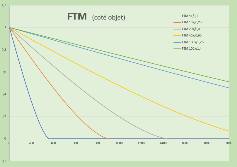
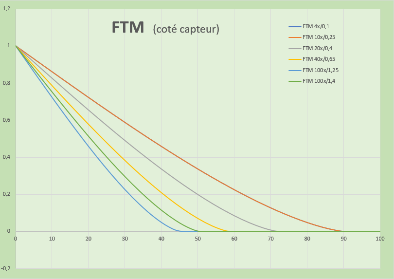
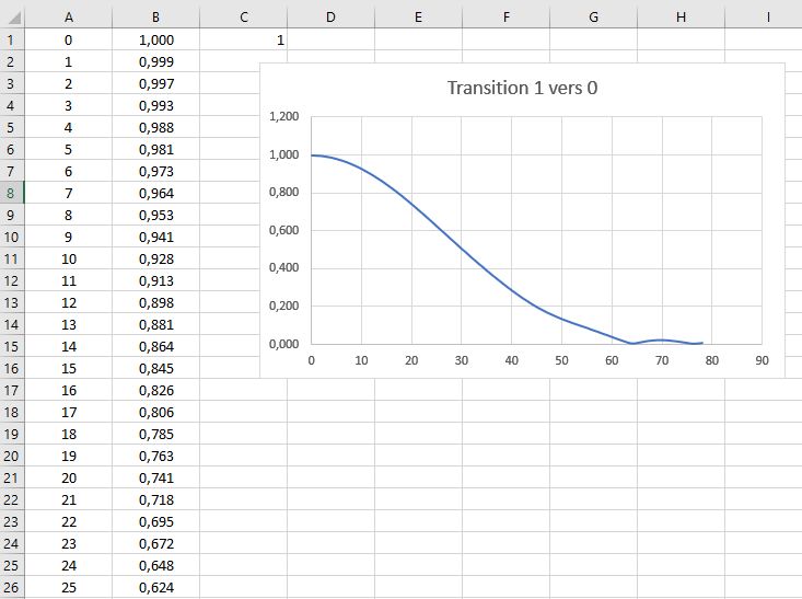
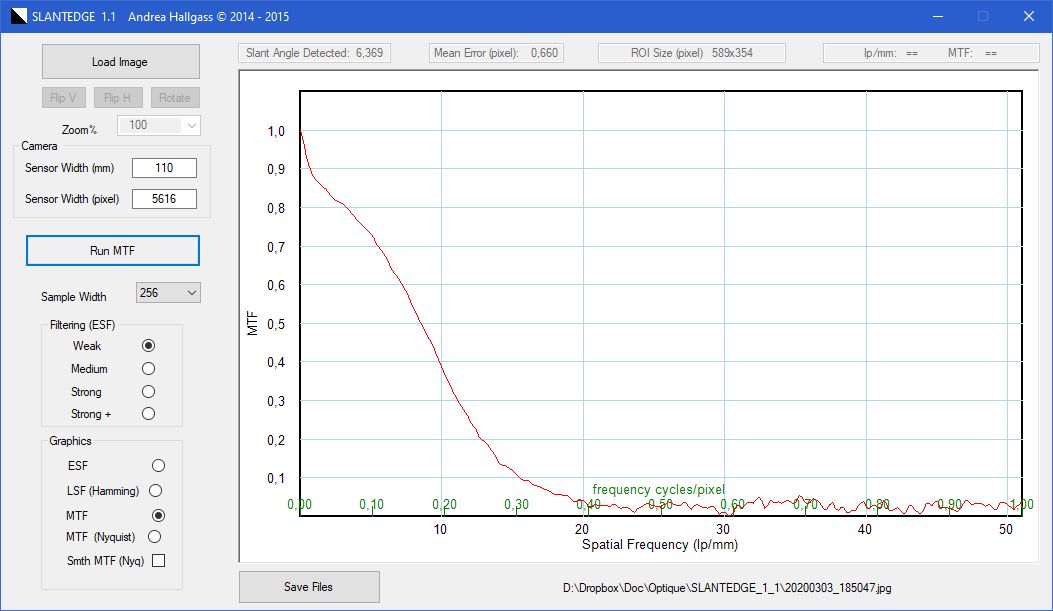
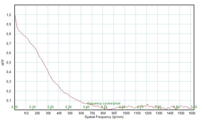
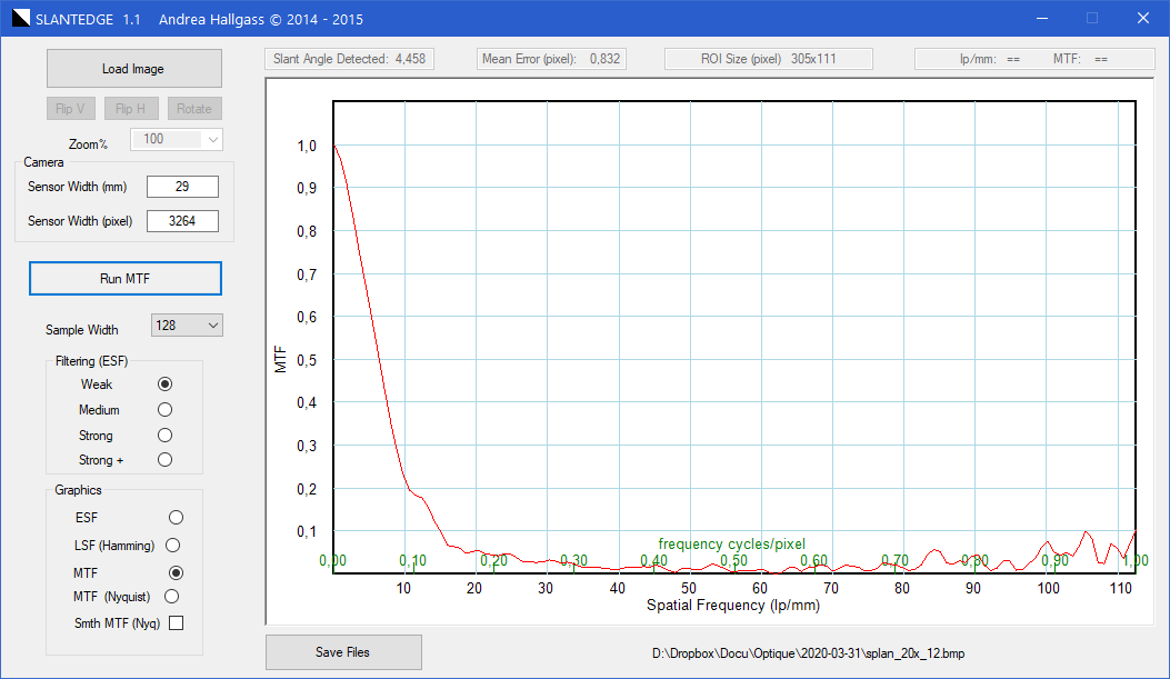
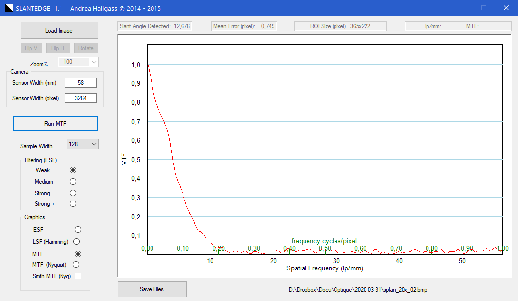
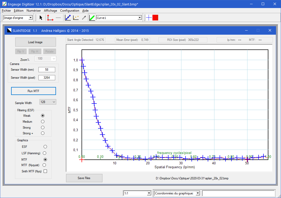
La FTM est à comparer à la bande passante souvent utilisée pour qualifier la qualité des appareils audio. En Audio on parle de Hertz=cycle/seconde. En Optique on parlera de FTM en lp/mm  (paire de lignes / mm)

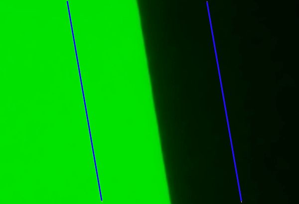
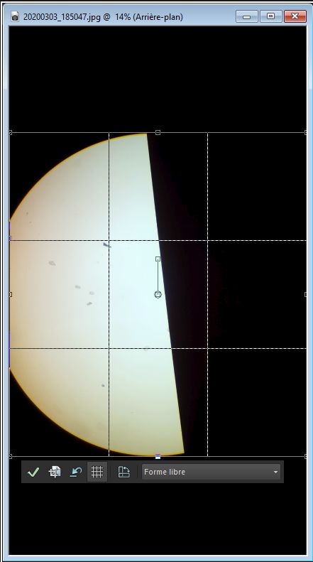
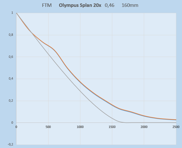
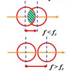
La théorie (complexe) pour établir la bande passante en optique (FTM) conduit à un résultat très étrange: La courbe est exactement celle de la lumière fournie par un système de 2 diaphragmes identiques que l'on décale!  Il s'agit donc de l'intersection de 2 cercles identiques dont les centres se décalent!  (autocorrélation de la fonction pupille)  (la partie verte-hachurée du dessin) 

FTM is to be compared to the bandwidth often used to qualify the quality of audio devices. In Audio we talk about Hertz=cycle/second. In Optics we talk about FTM in lp/mm (pair of lines / mm).

The (complex) theory to establish the bandwidth in optics (FTM) leads to a very strange result: The curve is exactly that of the light provided by a system of 2 identical diaphragms that are shifted!  It is thus the intersection of 2 identical circles whose centers are shifted!  (the green-shaded part of the drawing)

   La courbe théorique (parfaite) de la FTM est de cette forme:

The theoretical (perfect) FTM curve is of this shape:

Limite de fréquence Fc

Fc=2000 NA/lambda  est la fréquence de coupure de l'objectif. Au delà il n'y a que du bruit ou des artefacts inutiles.

Frequency limit Fc

Fc=2000 NA/lambda is the cut-off frequency of the lens. Beyond that there is only noise or useless artifacts.

 Le pied de chacune de ces courbes correspond au tableau du paragraphe précédent

Ces courbes peuvent être définies grossièrement afin d'éviter trop de caculs. On peut découvrir ces approximations utilisées lorsque les calculs se faisaient avec de faibles moyens ou à la main:  _Approximation_FTM.php

On peut remarquer que seuls les objectifs à faibles grossissements demandent des capteurs bien définis.

NB Les courbes 4x et 10x se superposent.

Les lois de l'optique sont valables dans toutes les directions, la vraie représentation de la FTM  doit se faire en 3D (voir figure ci dessous) Il s'agit donc d'une cône.

We can notice that only low magnification lenses require well defined sensors.

NB The 4x and 10x curves are superimposed.

The laws of optics are valid in all directions, the true representation of the MTF must be in 3D (see following figure). It is therefore a cone.

Que conclure de tout cela?: Eh bien, on en est qu'au début! Car rien ne nous permet de mesurer les caractéristiques d'un objectif à une fréquence donnée, puis de tracer des courbes...

What to conclude from all this: Well, we're only at the beginning! Because nothing allows us to measure the characteristics of a lens at a given frequency and then draw curves...

    Pour ceux qui ont fait un peu de maths, ils devraient se souvenir qu'il y a une relation entre les bandes passantes et les temps de montée d'un signal. En gros si on analyse les fronts des signaux on peut en déduire les BP, et réciproquement, si on connait les BP, on peut en déduire les fronts!

  Cette technique est utilisées dans les box ADSL. Un µP analyse le front, en déduit la BP, en déduit la correction de BP à effectuer, apporte un calcul de filtrage grâce à un DSP et ...  ce n'est pas le sujet de cet article!

 Ah!?, il y a un rapport entre la FTM et la forme d'une transition optique?     Eh oui!

Mais alors, il suffirait d'analyser une transition entre du noir et du blanc pour obtenir la qualité d'un objectif. OUI, OUI, OUI

Mais sous certaines conditions:

    J'ai commencé mes manips sans prendre conscience de ces conditions. Le reste de l'article ne sera donc pas parfait et devra être refait/relu/corrigé/modifié...

   For those who have done some math, they should remember that there is a relationship between bandwidths and signal rise times. Basically, if we analyze the signal fronts we can deduce the PBs, and conversely, if we know the PBs, we can deduce the fronts!

  This technique is used in ADSL boxes. A µP analyzes the edge, deduces the BP, deduces the BP correction to perform, provides a filtering calculation thanks to a DSP and ... this is not the subject of this article!  

Ah, there is a relationship between the MTF and the shape of an optical transition?     Yes there is!

But then, it would be enough to analyze a transition between black and white to obtain the quality of a lens. YES, YES, YES

But under certain conditions:

I started my manners without being aware of these conditions. The rest of the article will therefore not be perfect and will have to be redone/replaced/corrected/modified...

    C'est un problème majeur, car il faut une mire sans défaut, et bien noire. Pour le test d'objectifs macro ou autre on utilise des lames de rasoirs noircies au noir de fumée. L'examen de lames de rasoir montre que la ligne noire n'est pas régulière (qqs dents de scies)

Cela reste un point à améliorer. Chacun peut/doit donner des idées.

J'ai réfléchi à ce problème pendant pas mal de temps et j'ai fini par déduire qu'une surface aiguisée ne peut pas être de qualité (sauf à recourir à des pierres à aiguiser de luxe). Et puis un jour j'ai découpé un film plastique avec un couteau (on tend le plastique et on fait glisser le couteau)

Puis je me suis dit que cette technique devait être utilisée pour préparer des bandes magnétiques de VHS, ou K7. Bingo!

La solution (ma proposition)

- Prendre une planche à découper (ou tout autre plaque dure d'environ 15 cm de coté)

- Sacrifier une K7 audio dont le ruban est noir. 90 mn (pour avoir une faible épaisseur)

- Coller une extrémité du ruban sur la plaque (il faut que cela tienne bien, car on va légèrement tendre le ruban)

- Faire plusieurs boucle de ruban, en le tendant et en le plaquant, sans plis (le disposer avec un angle d'environ 5°) on peut facilement corriger l'angle par la suite.

   This is a major problem, because you need a flawless, black test pattern. For the test of macro lenses or other lenses we use razor blades blackened with smoke black. The examination of razor blades shows that the black line is not regular (some saw teeth).

This remains a point for improvement. Everyone can/should give ideas.

I have been thinking about this problem for quite some time and have come to the conclusion that a sharpened surface cannot be of quality (except by using luxury whetstones). And then one day I cut a plastic film with a knife (you tighten the plastic and slide the knife)

Then I said to myself that this technique should be used to prepare VHS tapes, or K7. Bingo!

The solution (my proposal)

- Take a cutting board (or any other hard board of about 15 cm on each side).

- Sacrifice a K7 audio tape whose ribbon is black. 90 mn (to have a low thickness)

- Stick one end of the ribbon on the plate (it must hold well, because we will slightly stretch the ribbon)

- Make several loops of ribbon, by stretching it and laying it flat, without folds (arrange it at an angle of about 5°) you can easily correct the angle afterwards.

- Prendre une lame vierge et polir tous ses bords avec une petite lime à ongles. C'est pour éviter de couper la bande magnétique qui est très fragile.

- Ayant pris soin de choisir une planche à découper avec rainures, je fais glisser la lame préparée sous les 4 bandes magnétiques. Cela permet de tendre un peu plus la bande, et on va pouvoir positionner la lame légèrement décalée (genre 5° vers la doite, 0h30) Le microscope va inverser l'angle ensuite pour le présenter à -5°/11h30 . Ce qui est réclamé par SlantEdge)

 - Take a blank blade and polish all its edges with a small nail file. This is to avoid cutting the magnetic strip which is very fragile.

- Having taken care to choose a cutting board with grooves, I slide the prepared blade under the 4 magnetic strips. This allows to tighten the tape a little more, and we will be able to position the blade slightly offset (like 5° to the right, 0h30) The microscope will invert the angle then to present it at -5°/11h30 . What is required by SlantEdge)

- Placer entre les bandes de tout petits points de colle UV de manière à prendre contact avec la lame et les lamelles. On cherche ici à obtenir une zone centrale (sans lamelles) pour faire des mesures en épi-scopie, et des zones avec du liant optique pour faire des mesures en dia-scopie. Il faut aussi que cela maintienne les rubans tendus en place.

 Attention: les points de colle doivent être petits, car la matière décompose le ruban. Ce qui est interdit. Il faut une transition parfaite au micron près. (Mes premiers essais ont été foireux!)

 - Place very small dots of UV glue between the strips so that they make contact with the board and the laminates. The aim here is to obtain a central area (without lamellae) for epi-scopic measurements, and areas with optical binder for dia-scopic measurements. This should also keep the ribbons taut in place.

Caution: the glue dots must be small, because the material will break down the tape. This is not allowed. A perfect transition to the nearest micron is required. (My first attempts were a failure!)

- Fixer le tout en appuyant sur les lamelles et en éclairant la colle UV avec la petite lampe UV. (Attention à ne pas perdre le très petit embout de la seringue 1mm x3mm, sinon le reste de la colle sera perdu)

- Fix it by pressing on the slats and illuminating the UV glue with the small UV lamp (be careful not to lose the very small tip of the 1mm x 3mm syringe, otherwise the rest of the glue will be lost).

  PS. J'ai effectué mes manips dans une véranda, avec toit en verre, et la colle a donc reçu rapidement des UV. Cela explique pourquoi une des lamelles est mal placée. (je l'ai vu trop tard)

PS. I did my maneuvers in a veranda, with a glass roof, so the glue received UV light quickly. This explains why one of the slats is misplaced. (I saw it too late)

  Cette disposition permet plusieurs zones: Epi-scopie au centre, avec lamelle sans colle, et avec lamelle avec liant optique.

- Une fois l'ensemble sec, éliminer les bouts de rubans avec un couteau ou lame de rasoir.

 This arrangement allows several zones: Epi-scopy in the center, with lamella without glue, and with lamella with optical binder.

- Once dry, remove the ribbon ends with a knife or razor blade.

Conclusion préparation de la lame

  On dispose maintenant d'une lame pour effectuer des mesures en épi et dia scopies. Elle est fragile car on peut accrocher les rubans. Tout le monde est capable de faire la même lame. Je n'ai pas de gélatine glycérinée, et je ne sais pas si on peut obtenir la même chose avec. A vous de faire des essais.

Le ruban doit être choisi le plus fin possible (k7 de 90 mn -> 10µm) et le plus noir possible . Le mien n'est que marron sombre, il me faudra refaire une lame de test.

Le ruban VHS doit être plus sombre. Ce sont des choses à essayer. Je vous laisse le faire.

A parté

Pour d'autres manips, je cherche à décoller la matière magnétique des rubans de K7 ou VHS? Quelqu'un aurait-il une idée simple, avec des produits communs, car je n'ai pas de produits chimiques à disposition.

 Conclusion slide preparation

  A slide is now available to perform measurements in epi and dia scopies. It is fragile because we can hang the ribbons. Everybody is able to make the same blade. I don't have glycerine gelatin, and I don't know if we can get the same thing with it. It's up to you to try.

The ribbon should be chosen as thin as possible (k7 of 90 mn -> 10µm) and as black as possible. Mine is only dark brown, I will have to redo a test slide.

The VHS tape should be darker. These are things to try. I'll let you do it.

Gone

For other maneuvers, I'm trying to peel the magnetic material from the tapes of K7 or VHS ? Would anyone have a simple idea, with common products, because I don't have any chemicals available.

Type de caméra

L'analyse fine de la transition noir-blanc impose d'utiliser une caméra présentant une densité de pixel élevée. J'utilise une caméra au format 1/2.3" de 8 MPx  ce qui offre une taille de pixel de 1.35 µm. tbc

Installation de la caméra

Elle doit être installée au foyer des optiques 160 mm ou au foyer de la lentille de tube pour les objectifs infinis.  On doit donc impérativement retirer tous les projectifs, relais, adaptateur, ... Rien ne doit se trouver entre la caméra (donc la surface du capteur) et l'objectif.

Dans les cas contraires, la mesure FTM obtenue serait le produit de 2 FTM: l'une de l'objectif, l'autre du système optique restant entre la surface du capteur et l'objectif.

Pour un système BHS, on peut trouver le plan foyer en démontant la partie haute de la sortie trinoculaire (3 vis à défaire et le foyer se trouve à environ 10 mm +intérieur d'un monture C) soit environ 25 mm

Le tirage mécanique est de 17,526 mm (0,69 pouce) pour une monture C, et 12,50 mm pour sa variante CS. wiki

- Démonter la partie supérieure du tube trino (3 vis Hexa)

- Mettre un adaptateur M42 à vis

- fixer la caméra (pistolet à colle)

Données à connaitre

Il sera nécessaire de connaitre la distance entre pixels de votre caméra, et évidemment sa définition.

Caméra utilisée dans cet exposé: DCM800

PC Interface  USB 2.0,support

Sensor 1/2.5 inch, Enhanced COLOR

CMOS , 8 M Pixels

Maximum Resolution  3264*2448 (Hardware)

Frame Rate : 1fps at 3264*2448,  30fps at 640*480

Capture Fram : Support high speed preview and static capture

Video Mode : 3264*2448,   1600*1200,   1280*768,   640*480

Dynamic Range : 75dB

Sensitivity : 1.3V/lux-sec  550nm .

Elle est beaucoup trop lente, et cela rend très difficile de faire le point.

Caméra idéale

Il existe maintenant des caméras prévues pour des postes de réparation de téléphones. Elles fournissent un flux HDMI de 30 ou 60 images/s Ce qui permet de voir en direct sur un écran la phase de réglage. Il en existe même des 4K ... beaucoup plus chères!

- 1/2.3" ou 1/2.5"

- hdmi pour visualiser en 1080*1920 en temps réel 30im/s

- 12 MPx ou 8 MPx

- Carte TF (micro SD pour des photos de qualité)

- télécommande  (pour ne pas avoir de bougé)

- USB3 impératif

- Capot métallique

- OS: win10

- Twain

- Save: BMP, jpg (très faibles pertes)

- Ne pas traiter le signal (pas de pré-accentuation)

- Sensible (il faudra prendre les clichés à 100 ISO, pour minimiser le bruit. Il faudra aussi beaucoup de lumière)

 Type of camera

The fine analysis of the black-and-white transition requires the use of a camera with a high pixel density. I use a 1/2.3" 8 MPx camera, which offers a pixel size of 1.35 µm. tbc

Camera installation

It must be installed at the focus of 160 mm optics or at the focus of the tube lens for infinite lenses.  It is therefore imperative to remove all the projectiles, relays, adapters, ... Nothing must be between the camera (so the sensor surface) and the lens.

Otherwise, the FTM measurement obtained would be the product of 2 FTM: one of the lens, the other of the optical system remaining between the sensor surface and the lens.

For a BHS system, we can find the focus plane by removing the upper part of the trinocular output (3 screws to undo and the focus is about 10 mm + inside a C-mount) or about 25 mm.

The mechanical draw is 17.526 mm (0.69 inch) for a C-mount, and 12.50 mm (0.69 inch) for its CS variant. wiki

- Remove the upper part of the trino tube (3 hex screws).

- Insert an M42 screw adapter

- fix the camera (glue gun)

Data to know

It will be necessary to know the distance between pixels of your camera, and obviously its definition.

Camera used in this presentation: DCM800

PC USB 2.0 interface, support

Sensor 1/2.5 inch, Enhanced COLOR

CMOS , 8 M Pixels

Maximum Resolution 3264*2448 (Hardware)

Frame Rate : 1fps at 3264*2448, 30fps at 640*480

Capture Fram: Support high speed preview and static capture

Video Mode : 3264*2448, 1600*1200, 1280*768, 640*480

Dynamic Range: 75dB

Sensitivity : 1.3V/lux-sec 550nm .

It is much too slow, and it makes it very difficult to take stock.

Ideal camera

Cameras are now available for telephone repair stations. They provide an HDMI stream of 30 or 60 fps which allows to see the adjustment phase live on a screen. There are even 4K cameras ... much more expensive!

- 1/2.3" or 1/2.5

- hdmi to view in 1080*1920 in real time 30 fps

- 12 MPx or 8 MPx

- TF card (micro SD for quality photos)

- remote control (so you don't have to move)

- USB3 imperative

- Metal cover

- OS: win10

- Twain

- Save: BMP, jpg (very low loss)

- Do not process the signal (no pre-emphasis)

- Sensitive (it will be necessary to take the shots at ISO 100, to minimize noise. You will also need a lot of light)

 Noter:
- Grandissement
- NA
- 160, 225 ou infini
- Compensation
- Présence lamelle
- Techno: epi/dia
- ChampH de la prise de vue en mm
- ChampH du capteur

Régler le microscope et la caméra. Vérifier qu'il n'y a pas de saturation.

Prendre une série de photo (genre stacking) en faisant varier la mise au point

L'enregistrer dans un répertoire normalisé

6.1- Utiliser le logiciel de recherche de la meilleure transition.
      (puis comprimer toutes les photos de la manip, et conserver un exemplaire de la bonne photo)
6.2- Extraire les données de cette transition.
6.3- Report dans la feuille de calcul  qui fera l'application de la correction gamma
      Vérifier la symétrie de la transition
6.4- Obtenir une transition moyennée
6.5- Calculer la meilleure approximation avec arc-tg + Gauss
6.6- Calcul de la dérivée  (pour compenser l'intégration initiale)
6.7- Calcul de la transformée de Fourier et de la FTM

  Je dispose d'un téléphone S6 Samsung facile à connecter sur mon BHS.

Il me donne des photos du style

 I have a Samsung S6 phone that is easy to connect to my BHS.

It gives me photos of the style

    Ne soyez pas choqué! C'est exprès!  On devine le diaphragme -> pour indiquer que le réglage du microscope doit être parfait. Le diaphragme sera légèrement agrandi par la suite.

  On devine le cercle indiquant le champ oculaire: c'est exprès, car il y aura des mesures de diamètres. On voit dans ce cercle un demi-cercle éclairé et un demi-cercle noir. Le tout avec un beau bord noir. Et cela a été difficile de fabriquer un beau bord noir. Il doit être franc, net, régulier, sans taches, ...  Car tout va se jouer sur la qualité/régularité de ce bord noir

  Mais cela ne va pas être possible!

Regardez la transition au niveau du pixel:  (ici 3 rangées de pixels)

 Don't be shocked! It's on purpose!  We guess the diaphragm -> to indicate that the microscope setting must be perfect. The diaphragm will be slightly enlarged afterwards.

  You can guess the circle indicating the eye field: this is on purpose, because there will be diameter measurements. We see in this circle an illuminated semicircle and a black semicircle. The whole with a beautiful black border. And it was difficult to make a nice black border. It must be frank, clean, regular, without spots, ...  Because everything will depend on the quality/regularity of this black border.

  But this is not going to be possible!

Look at the transition at the pixel level: (here 3 rows of pixels)

  La transition se fait sur une dizaine de pixels, et le signal va être en forme d'escalier (non continu) Impossible de faire une analyse avec un signal très grossier.  J'ai perdu mon temps. (?)

Puis au fil des jours on se dit qu'on doit pouvoir améliorer les choses: J'ai plusieurs milliers de transitions dans mon image. Ne peut-on faire une analyse statistique?

 The transition is done on about ten pixels, and the signal will be in the shape of a staircase (not continuous). It is impossible to make an analysis with a very coarse signal.  I wasted my time. (?)

Then, as the days go by, we tell ourselves that we should be able to improve things: I have several thousand transitions in my image. Can't we do a statistical analysis?

  On va détecter l'orientation de la figure, tracer un canal, et faire une analyse statistique dessus.

  Reste le problème des 10 pixels du motifs. Il faudra multiplier cela par au moins x25 !

Je vais alors utiliser une méthode ancienne (que j'ai découvert il y a 50 ans) qui permettait d'analyser des signaux répétitifs de 5 GHZ avec des oscilloscopes de 100 MHz.  D'une trace à l'autre on décalait  les signaux de 0.1 nS...  (approx)

  Dans le cas présent cela se traduit par légèrement décaler le canal d'analyse, et magiquement, d'une manièe synthétique on obtient une transition sur 256 pixels!  Et cela permet maintenant de faire des calculs de Fourier (passer de transition à FTM)

  Calculs compliqués, surtout à mon age, erreurs en cascades, bidouilles, simplification, découvertes de plein de méthodes inconnues, de langages, ... une vraie quête du Graal!

 We will detect the orientation of the figure, draw a channel, and do a statistical analysis on it.

  There remains the problem of the 10 pixels of the pattern. We will have to multiply this by at least x25!

I will then use an old method (which I discovered 50 years ago) which allowed me to analyze repetitive signals of 5 GHZ with 100 MHz oscilloscopes.  From one trace to another, the signals were shifted by 0.1 nS...  (approx)

  In this case this translates into a slight shift of the analysis channel, and magically, in a synthetic way we get a transition on 256 pixels!  And this allows now to do Fourier calculations (to switch from transition to FTM).

  Complicated calculations, especially at my age, cascading errors, tinkering, simplification, discovery of many unknown methods, languages, ... a real quest for the Grail!

  Et tout d'un coup j'ai trouvé LA solution: Quelqu'un de beaucoup plus jeune avait fait le travail!

Mais il restait à l'adapter à la microscopie.

 And suddenly I found THE solution: Someone much younger had done the job!

But it still had to be adapted to microscopy.

 On cherche la FTM du coté objet. Ce sera pour vérifier que l'objectif est de précision et a bien une acuité de 1.1 µm.

1,1 µm =Lambda/2*NA     avec Lambda=0.55µm   NA=0.25   G=10x

Il faut retranscrire les données du capteur au niveau de l'objet, car on cherche le nombre de paire de ligne au niveau de l'objet (de la lame ou de l'échantillon)

Dans le cas du téléphone S6, on a le cercle qui tangente

On va mesurer (en pixels) le diamètre du cercle.

                ici  3263 px

Avec une lame de référence on va mesurer le diamètre en mm

[au pif, sachant que le champ oculaire est de 26.5 mm, et que le grandissement de l'objectif est 10x.

Le champ au niveau de l'objet/lame sera de 26.5/10 =2.65 mm]

On pourra dire que le capteur fait 2.65mm pour  3263 px. Valeurs que l'on reportera dans le logiciel.

En réalité on reportera 26.5mm  et 3263 px sachant qu'il faudra multiplier par 10x la lecture de l'abscisse lp/mm  (car sinon les chiffres se superposent)

NB Manips avec PSP

We will measure (in pixels) the diameter of the circle.

                 here 3263 px

With a reference slide we will measure the diameter in mm

[at random, knowing that the field of view is 26.5 mm, and that the magnification of the objective is 10x.

The field at the object / blade will be 26.5/10 = 2.65 mm]

We can say that the sensor is 2.65mm for 3263 px. Values that will be transferred to the software.

In reality we will transfer 26.5mm and 3263 px knowing that it will be necessary to multiply by 10x the reading of the abscissa lp/mm (because if not the figures overlap)

NB Manips with PSP

 L'importance des mesures et évaluations.
Une erreur de 10 % sur la mesure du diamètre introduit une errer de 10 % dans la fréquence de coupure de la MTF! Exemple, j'ai pris ci-dessus l'hypothèse d'avoir un champ de 2.65mm. En réalité je n'ai que 2.0 mm.

 Objectif MSplan 10x Olympus, lumière LED blanche, Champ 2 mm et 3263 px (montage BHS avec équipement EPI)

(Les chiffres verts ne sont pas corrigés. LP corrigés.   20200303_185047.jpg) Attention: Sur le téléphone S6, si on utilise la loupe pour affiner la mise au point, il faut penser à revenir à la fonction x1 pour voir le cercle entier. sinon cela ne fonctionne pas.

  Attention: les images affichées ne correspondent pas toujours aux manips expliquées. J'ai fait plein de capture et ai fini par me mélanger les idées/images.

Le cycle de mesure comporte plusieurs phases:

80- Régler la caméra et l'angle de la lame

81- Capture d'une série d'images par stacking en format bmp : Les artefacts du jpg ne sont pas acceptables (après avoir bien réglé son microscope)

82- Rechercher la meilleure image/zone avec mon logiciel FTM_SlantEdge

83- Calculer la FTM avec SlantEdge  (il faudra obtenir un image en bmp)

83- Passage dans Engauge pour obtenir les valeurs numériques de la FTM mesurée par SlantEdge.

84- Normaliser les données avec mon programme Excel. Cela permettra à ce stade de comparer plusieurs objectifs/courbes

 Warning: the images displayed do not always correspond to the explained manners. I did a lot of capturing and ended up mixing up the ideas/images.

The measurement cycle has several phases:

80- Adjusting the camera and the angle of the blade

81- Capturing a series of images by stacking in bmp format: The jpg artifacts are not acceptable (after having properly adjusted your microscope)

82- Search for the best image/area with my FTM_SlantEdge software

83- Calculate the TMT with SlantEdge (you will need to get a bmp image)

83- Switch to Engauge to obtain the numerical values of the MTF measured by SlantEdge.

84- Normalize the data with my Excel program. This will allow at this stage to compare several objectives/curves

  Il est important de bien régler sa caméra avec de bonnes conditions de lumière. Il faut que la partie noire soit à gauche, et que la partie blanche ne soit pas saturée. Le contraste ne doit pas être trop grand (car la 'continuité' de la fonction gamma sera en défaut)

  Un des problèmes important est de garantir un bon S/B dans la partie éclairée/blanche. Il faut donc beaucoup de lumière et régler sa caméra en faible sensibilité: genre ISO 100. Le temps de capture de l'image sera assez grand (genre 0.5 s)

  La lame doit être orientée à environ 7°  (comme l'aiguille des heures à 11h45   Car 11h->90/3=30°  11h30->15°  11h45->7.5°  )

 It is important to set up your camera with good lighting conditions. The black part must be on the left, and the white part must not be saturated. The contrast should not be too high (because the 'continuity' of the gamma function will be defective).

An important issue is to ensure good S/B in the lit/white area. So you need a lot of light and set your camera in low sensitivity: like ISO 100. The image capture time will be quite long (like 0.5 s).

The blade must be oriented at about 7° (like the hour hand at 11:45 am because 11h->90/3=30° 11h30->15° 11h45->7.5° )

- Régler parfaitement son microscope: condenseur, diaphragme, point, éclairage.

- La netteté doit être parfaite (et c'est le point que je trouve le plus délicat) Car la mesure de la FTM impose un point parfait. Un simple décalage de lambda=0.55µm minimise la courbe. Il faudra faire plusieurs clichés correspondants à plusieurs mises au point.

La bonne méthode consiste donc à faire du satcking pour être certain d'avoir une zone avec mise au point parfaite. Un lot de 10 à 15 images est un bon choix.

- Chacun utilisera son logiciel habituel de capture, en bmp couleur.  (vous pourrez ensuite archiver vos images avec PkZip ou WinRar. Il y aura un très forte compressionbcar les images sont sans motifs)

- Chacun devra noter les caractéristiques de la caméra utilisée et de l'objectif en test. Il sera préférable de regrouper une expérience sur un répertoire particulier. (genre:  Splan_10x)

 - Adjust your microscope perfectly: condenser, diaphragm, point, illumination.

- The sharpness must be perfect (and this is the point that I find the most delicate) because the measurement of the FTM imposes a perfect point. A simple shift of lambda=0.55µm minimizes the curve. It will be necessary to make several shots corresponding to several settings.

The good method is therefore to do satcking to be sure to have a zone with perfect focus. A batch of 10 to 15 images is a good choice.

- Each one will use his usual capture software, in bmp color (you can then archive your images with PkZip or WinRar. There will be a very strong compression because the images are without patterns).

- Everyone will have to note the characteristics of the camera used and the lens under test. It will be preferable to group an experiment on a particular repertoire. (like: Splan_10x)

  Pour déterminer la meilleure zone à utiliser/fournir à SlantEdge

Ce programme va analyser (avec votre aide) la série de photos prises en format *.bmp. Vous devrez regarder toutes les photos, faire varier le seuil pour repérer les meilleures zones.

82o- Vérifier vos photos: lot en bmp, définition max, partie noire à gauche, format horizontal, inclinaison 11h45, noir et blanc. Sinon refaire!

82a- Lancer le programme

 To determine the best area to use/supply to SlantEdge

This program will analyze (with your help) the series of photos taken in *.bmp format. You will have to look at all the photos, vary the threshold to find the best areas.

82o- Check your photos: bmp batch, max definition, black part on the left, horizontal format, tilt 11:45, black and white. If not, do it again!

82a- Launch the program

82b- Initialiser les répertoires en allant dans le menu Installation. Indiquer les définitions de votre caméra. (il me faudra connaitre vos caméras pour faciliter l'affichage des définitions. Pour l'instant cela se limite à MA caméra!)

82c- Analyser le lot d'images

 82b- Initialize the directories by going to the Installation menu. Indicate the definitions of your camera (I will need to know your cameras to facilitate the display of the definitions. For the moment this is limited to MY camera).

82c- Analyze the batch of images

 The program has been adapted for 100% SlantEdge operation which details your image in 5 screens. I made green lines appear delimiting these 5 screens of 100% SlantEdge.

My program detects image transitions (black area on the left) and performs statistics to identify the largest areas with the steepest transitions (these are the areas that are the sharpest).

If you look at the image above, you will find the sharpest area in the SlantEdge100% screen at the top and you will need to select the corresponding yellow area. Here this area contains 130 contiguous TV lines.    Image to select: 18.bmp

By varying the threshold, even finer zones can be determined.

82x- Conclusions: This program allows you to detect the best image and indicates which is the best sharpness zone.  It also verifies if you are using the maximum definition of your sensor.

82 PS- The white area of your images is completely hidden (as soon as the transition is detected) to facilitate the readability of my program. The transition area beyond the threshold is indicated by colored cyan dots.

 Caméra   3264*2448  Dimension: 5.8 mm horizontal  Pixels: 1.35 µm    (0.135 µm sur l'objet si obj_10x)

MS plan 10x 0.25  (si capteur sans relais)
    résolution objet= 1,1 µm =Lambda/2*NA
    Tache capteur=     11 µm =G * Lambda /(2*NA)
    Pixel limite = 5,5 µm   

0- Régler SlantEdge en fonction des tailles capteurs, définition, ...

Comme SlantEdge n'accepte pas 0.58 mm = 5.8 mm/Grossissement  on indiquera on valeur 100x supérieure, sachant que l'axe des x sera à multiplier par 100x  (10x pour compenser la taille du capteur, et x10 pour le grandissement de l'objectif. Le programme Ecel effectuera ces corrections)

1- retourner la photo (si nécessaire) jusqu'à avoir le noir du coté gauche

0- Adjust SlantEdge according to sensor sizes, definition, ...

As SlantEdge does not accept 0.58 mm = 5.8 mm / Magnification, we will indicate a value 100x higher, knowing that the x-axis will be multiplied by 100x (10x to compensate for the sensor size, and x10 for the lens magnification). The Ecel program will make these corrections)

1- flip the photo (if necessary) until black on the left side

 C'est vraiment facile à faire!

5- Sauver la fenêtre de SlantEdge en bmp

Sur Win10 je fais:

      sélection de la fenêtre SlantEdge > AltGraph-ImpressionEcran > Lancer Irfan view > copier dans Irfanview > sauver en bmp.

Il faut sauver en bmp pour ne pas avoir d'arrondis. Ces images volumineuses pourront être détruites en fin de manips. On peut n'enregister que la courbe avec ses axes: Sous IrfanView > sélection zone > Ctrl-Y > Ctrl-S

x- Fin SlantEdge    

 A ce stade nous disposons d'une image codée bmp qui représente la courbe obtenue par SlantEdge.

5- Sauver les données fournies par SlantEdge

Sélection de MTF > Save Files      qui va créer un fichier texte  avec le même nom que l'image analysée.

x- Fin SlantEdge    

5- Save the data provided by SlantEdge

 Prendre mon programme _SlantEdge_FTM.xls   Il faut préciser les caractéristiques de l'objectif et de la caméra  (cases vertes, en haut)

On remarquera que les cases vertes indiquent les endroits où on peut changer les valeurs, en bleu-ciel les résultats de calculs, en saumon: titres de sections

Ce programme va reprendre toutes les données et effectuer de nombreuses interpolations afin de faciliter la comparaison d'optiques. En gros on va recalculer les valeurs pour des abscisses entières genre 1  2  3  .. 10  11  etc (Car les données fournies par Engauge ne sont pas arrondies)  (Fonctions devenues inutiles)

Méthode

Copier les données numériques fournies par SlantEdge : 

sélection >  crtl-c, et les copier dans la case A2 avec ctrl-v  (ou A1 si vous avez le texte du haut)

Convertir: L'action suivante mettra les données sur 2 colonnes:  

 Tout cela semble compliqué  s'est beaucoup simplifié, mais avec un peu d'apprentissage, cela devient très rapide.

Mise au point µScope> Photo bmp > Analyse des photos > MTF avec SlantEdge >  Excel

Le cycle de mesure comporte plusieurs phases:

91- Préparation et réglages du microscope et de la caméra

92- Capture de plusieurs images en format bmp   (pas d'artefact de jpg)

93- Sélectionner la meilleure image et la meilleure zone avec mon programme

94- Obtenir la meilleure FTM brute avec SlantEdge  (export en txt)

94- Passage dans Engauge pour obtenir les valeurs numériques de la FTM mesurée par SlantEdge.

95- Normaliser les données avec mon programme Excel. Cela permettra à ce stade de comparer plusieurs objectifs/courbes

 The measurement cycle consists of several phases:

91- Preparation and adjustments of the microscope and the camera

92- Capturing multiple images in bmp format (no jpg artifact)

93- Select the best image and the best area with my program

94- Get the best raw FTM with SlantEdge (export in txt)

94- Switch to Engauge to obtain the numerical values of the MTF measured by SlantEdge.

95- Normalize the data with my Excel program. This will allow at this stage to compare several objectives/curves

La mesure de la qualité d'un objectif impose que le microscope soit parfaitement réglé:

- Positionner le condenseur 

- vérifier aussi le centrage de la lumière- Régler le diaphragme (l'ouvrir juste à la disparition)  (cela évitera les éblouissements)

- Régler maintenant la caméra qui doit être parafocale avec le reste. (sans toucher aux réglages précédents)  donc réglage mécanique

- Régler la caméra au niveau photo: balance des blancs, exposition, quantité de lumière, etc.

Measuring the quality of an objective requires the microscope to be perfectly adjusted:

- Position the condenser

- Set the test pattern and focus on the part corresponding to the objectives (lamella, or episcopy).

- Close the diphragm a little to see it. Center it

- raise/lower the condenser plate to clean the diaphragm

- check also the light centering - adjust the diaphragm (open it just to disappear) (this will avoid glare)

- Now set the camera that should be parafocal with the rest. (without touching the previous settings) so mechanical adjustment

- Set the camera to photo level: white balance, exposure, amount of light, etc.

  Il va falloir prendre une série de photos comme en stacking pour être certain d'avoir un cliché comportant une mise au point parfaite. Mon logiciel analysera toutes les photos et vous permettra de connaitre la bonne photo à utiliser et la zone où la netteté sera parfaite.

- La partie noire devra être à gauche, et la transition devra faire un angle de 7°   (entre 11h30 et 11h50) et cela demande à faire attention! Sinon refus!

- Les photos seront prises dans le standard BMP et en Couleur. (pas de jpg!)  Elles auront la définition maximale. Et devront être nommées en fonction de l'objectif. Ex Splan_10x_01.bmp . Ou plus simplement nommer un répertoire du nom de l'objectif et laisser votre logiciel de capture proposer un nom (ce sera plus rapide) Il faut garantir un faible bruit dans les parties claires. (voir les paragraphes précédents)

 - Régler la prise de vue (sur écran de votre PC. C'est l'écran/caméra qu'il faut regarder!) un peu avant la netteté et prendre un cliché en BMP. (puis modifier la mise au point)  Il faut donc entourer la zone de netteté.

 NB Il faudra apporter un soin très particulier à ne pas saturer la partie droite de l'image. Un test sera fait qui rejettera les photos avec une partie droite saturée. (Car cela interdit de calculer une FTM sérieuse)

 You will have to take a series of photos as in stacking to be sure to have a picture with perfect focus. My software will analyze all the photos and will let you know the right photo to use and the area where the sharpness will be perfect.

- The black part should be on the left, and the transition should be at an angle of 7° (between 11:30 and 11:50) and this requires attention! Otherwise, refuse!

- The photos will be taken in BMP standard and in Color. (no jpg!) They will have the maximum definition. And will have to be named according to the objective. Ex Splan_10x_01.bmp. Or more simply name a directory with the name of the lens and let your capture software propose a name (it will be faster). It is necessary to guarantee a low noise in the clear parts. (see previous paragraphs)

- Adjust the shot (on your PC screen, it's the screen/camera you have to look at!) a little before sharpening and take a BMP shot. (and then change the focus) You must therefore surround the sharpness area.

NB It will be necessary to take a very particular care not to saturate the right part of the image. A test will be made which will reject photos with a saturated right part. (Because this prohibits to calculate a serious FTM)

  Utiliser mon logiciel qui analysera toutes les photos et vous permettra de connaitre la bonne photo à utiliser et la zone où la netteté sera parfaite.

(dev en cours... Résultats très prometteurs)

Il comporte un analyseur de transition, Une fonction de dérivation, puis recherche de polynômes Gaussiens de la dérivée, pour reconstitution interpolative par intégration, pour obtenir une FFT avec forte définition. Série de Gauss et de fonctions de Fermi)

 Use my software that will analyze all the photos and let you know the right photo to use and the area where the sharpness will be perfect.

(dev in progress... Very promising results)

It includes a transition analyzer, a derivation function, then search for Gaussian polynomials of the derivative, for interpolative reconstruction by integration, to obtain a FFT with high definition. Series of Gaussian and Fermi functions)

 et analyser la photo sélectionnée dans le paragraphe 93.

Régler SlantEdge:   

1- Sensor Width=Dim h de votre capteur x10 (ici 5.8 mm x10=58)            

2- Définition de votre capteur (ici 3264 pixels H)

3- Zoom 100

•  Repérer la meilleure zone de la photo (on prendra par ex, le meilleur résultat pour la 4eme colonne. ici 0.25)

• Vérifier qu'il n'y a pas de saturation en regardant la courbe ESF

• Une fois repérée la bonne zone de la photo, sauvegarder les données de SlantEdge avec le réglage MTF Nyquist

•  Prendre mon programme _SlantEdge_FTM.xls   Il faut préciser les caractéristiques de l'objectif et de la caméra  (cases vertes, en haut)

• Recopier les données fournies par SlantEdge

En orange: FTM pure

En bleu FTM brute (avec influence du capteur)

On remarque très peu de différences: Cela est dû au capteur utilisé sans adaptation optique (pas de relais)

L'objectif a une résolution de 0.9 µm et on l'échantillonne avec un pas de 0.175 µm. Soit plus de 5 pixels par dot.

Nyquist n'en demande que 2 (3 est mieux)

Il reste à étudier l'influence du filtre AA Anti-Aliasing. Mais rien ne dit qu'il y en a un! (Pas de specs du capteur).

In orange: pure FTM

In blue: raw FTM (with sensor influence)

We notice very few differences: This is due to the sensor used without optical adaptation (no relay)

The lens has a resolution of 0.9 µm and is sampled with a step of 0.175 µm. That is more than 5 pixels per dot.

Nyquist requires only 2 (3 is better)

It remains to study the influence of the AA Anti-Aliasing filter. But nothing says that there is one! (No specs of the sensor).

 Attention: L'objectif Splan est un objectif qui demande compensation. Le manque de compensation se retrouve donc dans la courbe FTM.

Note générale:   J'ai effectué énormément de mesures. Les courbes, tableaux présentés dans ce document, ne se correspondent pas! j'ai pris dans mon stock, au hasard, pour illustrer ce document

 Sans compensation. Tests effectués avant la création de mon programme

97a- prise de 12 clichés en faisant varier la mise au point (dans le même sens) comme si je faisais du stacking.

@0.xx correspondent aux abscisses vertes cy/pixel  (pris comme simple repère)

 97f- Passage dans Excel:

- Ouvrir mon programme

- ouvrir le csv avec notepad ou Textpad. > sélectionner la zone des données

- Recopier dans la cellule A1 de Excel

 - Admirer la courbe obtenue et prenez l'apéro!

Conclusion: Il est impératif de mesurer cet objectif avec un projectif!  La courbe ne devrait pas passer au dessus de la FTM théorique (grise)

L'analyse de cette courbe montre 2 problèmes:

1- L'arrondi au début est dû à une mauvaise utilisation d'Excel (il ne faut pas prendre l'option courbe avec spline)

2- Le passage par dessus le pied de la courbe (en bas) Cela est dû au fait que SlantEdge ne tient pas compte du gamma des images.  La courbe ici est très optimiste

 - Cela fonctionne bien et permet de comparer des objectifs.

- Attention aux objectifs compensés: Il va falloir faire les mesures avec un projectif certifié.
Il va donc falloir adapter nos mesures: Si non compensation (comme les Cnscope) la méthode ci-dessus est valable. Si on veut mesurer des objectifs compensés il faudra faire les manips avec un couple objectif-projectif.

- La comparaison de mes tests faits avec smartphone et caméra au foyer indique/démontre/ suspecte que le smartphone triture la FTM de l'objectif. C'est tout un pan de mesure et d'essais à faire/analyser. Je suspecte (pratiquement sûr) que la BandePassante/FTM triangulaire est corrigée pour devenir rectangulaire. (Comme une correction des aigus en audio)    Cela expliquerait pourquoi une photo prise avec mon téléphone est bien meilleure, et que la courbe mesurée se trouve en dehors de la zone théorique de la FTM.  (suspicion forte de l'oubli que les images sont codées dans un espace gamma=0.5  <- Je viens de prouver ce fait. SlantEdge ne tient pas compte du gamma)

- Il me faut trouver une solution pour faire une mire sans dissolution de la piste magnétique. (Gélatine glycérinée?)

- lame de rasoir adoucie avec pierre à 0.2µm ?

- This works well and allows you to compare lenses.
- Be careful with compensated lenses: We will have to make the measurements with a certified projector.

We will have to adapt our measurements: If not compensated (like Cnscope) the above method is valid. If we want to measure compensated lenses, we will have to make the manips with a couple of lenses.
- The comparison of my tests made with smartphone and camera in focus indicates / demonstrates / suspects that the smartphone is manipulating the FTM of the lens. That's a whole bunch of measuring and testing to do/analyze. I suspect (pretty sure) that the triangular BandPass/FTM is corrected to rectangular. (Like a treble correction in audio) This would explain why a photo taken with my phone is much better, and the measured curve is outside the theoretical FTM area. (Strong suspicion of forgetting that images are coded in a gamma=0.5 space <- I just proved this fact. SlantEdge does not take gamma into account)

- I need to find a solution to make a test pattern without dissolving the magnetic track. (Glycerine gelatin?)

- razor blade softened with 0.2µm stone?

- Automate the measurements... in progress and partially solved.

 SlantEdge a été étudié/créé pour analyser des objectifs classiques genre 50 mm, 90 mm, 105 mm. Objectifs d'usage commun avec des full-frames (35mm) ou APS-c.

 Dans le cas des objectifs de microscope, et compte tenu qu'il faut un taux d'échantillonnage élevé, les caméras n'ont qu'une faible surface (ou faibles dimensions)

SlantEdge va donner des courbes illisibles/inexploitables. Ex pour un capteur 1/2.5" 1.75µm 3264 pixels horizontaux

 Reprenons la même photo/zone mais en supposant un capteur 10x plus grand: sensor=58 mm, et toujours 3264 pixels de longueur. L'axe des x (ou axe des fréquence devient lisible, mais il est faux, puisqu'on a multiplié par 10 la taille du capteur. Il faut donc corriger cet axe en multipliant par 10 les valeurs:

Let's take the same picture/area but assuming a 10x larger sensor: sensor=58 mm, and still 3264 pixels long. The x-axis (or frequency axis) becomes readable, but it is false, since we have multiplied by 10 the size of the sensor. We must therefore correct this axis by multiplying by 10 the values:

 La fréquence au capteur doit donc être multipliée par 10x (pour compenser le facteur du grossissement fictif x10 du capteur)

 Ce qui nous intéresse est de connaitre le piqué de l'objectif au niveau de la source. Il s'agit bien du pouvoir séparateur de l'objectif. Or on a analysé que la fréquence spatiale au niveau du capteur. (dimensions du capteur, taille du pixel, définition du capteur. L'objectif n'est pas intervenu. SlantEdge n'a aucune connaissance de l'objectif. Il ne peut que déduire une fréquence spatiale d'une image)

Pour ramener l'expérience au niveau de la source, il faudra multiplier la fréquence spatiale par le grandissement de l'objectif. Ici il faudra multiplier par 20x puique l'objectif est un Splan 20x

Pour résumer les corrections à apporter:

-  x10 pour compenser la petite taille du capteur

-  x20 pour ramener au pouvoir séparateur de l'objectif.

Résumé de ce qu'il faut faire:

- Multiplier par x10 la taille réelle du capteur (et toujours conserver cette dimension. Elle ne varie pas en fonction des objectifs à tester)

What interests us is to know the sharpness of the lens at the source. This is the separating power of the lens. But we analyzed that the spatial frequency at the sensor. (dimensions of the sensor, pixel size, definition of the sensor. The lens did not intervene. SlantEdge has no knowledge of the lens. It can only deduce a spatial frequency of an image)

To summarize the corrections to be made:

Summary of what to do:

 Evidemment mon programme Excel fait ces corrections.

 J'ai trouvé l'erreur: l'original ne fait pas la bonne taille (caméra mal réglée) Image 1600x1200 au lieu de 3264x2448. Cela fausse donc le calcul de SlantEdge.  Il faudrait /2 les valeurs.

Conclusion: mon logiciel détectera/vérifiera la taille des photos

 L'idée était de mesurer l'impact de la compensation. Pour cette mesure, le microscope était installé en dia-scopie, mais sans lamelles (noLame)   Même montage pour les 3 mesures. (pas de NFK)

Description des noms

4x: Grandissement de l'objectif

0.1 ou 0.13 : ouverture. NA=0.1 objectif simple   NA=0.13 objectif semi-apo   (obj en 160mm)

WLame: avec lamelle    NoLame=Sans lamelle

K: avec compensation   NoK=sans compensation (pas de projectif NFK)

xx.bmp  Ref de la photo présentant la meilleure transition.

NB: Faire une comparaison compensation/sans compensation impose de faire 2 montages différents. Un des 2 imposant l'usage d'un projectif compenseur NFK. Cela impose de recalibrer le capteur...

Description of names

4x: Lens magnification

0.1 or 0.13: opening. NA=0.1 single lens NA=0.13 semi-apo lens (obj in 160mm)

WLame: with lamellae           NoLame=Without lamellae

K: with compensation             NoK=without compensation (no NFK relay)

xx.bmp Ref of the photo with the best transition.

NB: To make a comparison between compensated and uncompensated photos, you have to make 2 different edits. One of the 2 requires the use of a NFK compensating projectile. This imposes to recalibrate the sensor...

fig. Une des courbes donne la qualité sans lamelle

On peut déduire de tout cela ( et d'autres manips) que le JML est un 20x NA=0.3?, 215mm, métallo.(et qu'il est moins bon que le Splan 20x)

fig. One of the curves gives quality without lamellae

We can deduce from all this (and other works) that the JML is a 20x NA=0.3?, 215mm, metallo (and that it is not as good as the Splan 20x).

Bon, tout cela représente des mesures préliminaires, qui demandent à être refaites avec la nouvelle caméra et mes nouveaux programmes. (je peux avoir fait des erreurs) Il faudrait qu'une autre personne refasse les mêmes mesures pour vérifier la validité... 

  fig. Superiority of the Splan

Well, these are all preliminary measures, which need to be redone with the new camera and my new programs. (I may have made mistakes) Someone else would have to redo the same measurements to check the validity...